Wednesday, June 24, 2009
Display problem ? Click HERE
Recommended :
Subscribe FREE - Chemical Processing
 Chemical Engineering has shared a FAYF related FLUID FLOW. This FAYF is infact has been released in previous month, however, CE share with CE FREE subscriber again this month.
Fluid Type
In this FAYF, it starts with definition of fluid type such as :
i) Newtonian
ii) Power law
iii) Bingham plastic
where
Newtonian fluid
A fluid is known to be Newtonian when shear stresses associated with flow are directly proportional to the shear rate of the fluid.
Power law fluid
A structural fluid has a structure that forms in the undeformed state, but then breaks down as shear rate increases. Such a fluid exhibits “power law” behavior at intermediate shear rates
Bingham plastic fluid
A plastic is a material that exhibits a yield stress, meaning that it behaves as a solid below the stress level and as a fluid above the stress level
This one-page fact sheet summarizes information pertinent to laminar and turbulent pipe flow for the various types of fluids commonly encountered in the CPI...
Ref. :
1. Darby, R., Take the Mystery Out of Non-Newtonian Fluids, Chem. Eng., March 2001, pp. 66–73.
2. Churchil, S. W., Friction Factor Equation Spans all Fluid- Flow Regimes, Chem. Eng., November 1997, p. 91.
3. Darby, R., and Chang, H. D., A Generalized Correlation for Friction Loss in Drag-reducing Polymer Solutions, AIChE J., 30, p. 274, 1984.
4. Darby, R., and Chang, H. D., A Friction Factor Equation for Bingham Plastics, Slurries and Suspensions for all Fluid Flow Regimes, Chem. Eng., December 28, 1981, pp. 59–61.
5. Darby, R., “Fluid Mechanics for Chemical Engineers,” Vol. 2, Marcel Dekker, New York, N.Y., 2001.
Download (Only for FREE CE Subscriber)
Note :
*This FAYF is only available FREE to Chemical Engineering Magazine registered user. Login required. Subscribe FREE CE, click here.
** Download immediately as article available FREE within short period only. Do not wait.
*** Found lost link or unable to download, may contact me...
Related Topic
Labels: Fluid Flow
Monday, June 22, 2009
Display problem ? Click HERE
Recommended :Liquefied Natural Gas (LNG) is one of the cleanest energy among all other energy sources.LNG and Supply Chain discussed briefly entire production, transportation, receiving and distribution path of LNG. There are still many peoples who are safety, environment & security concerns, not agreeing with the LNG production as discussed in "LNG SES Issues...".
Liquefy Natural gas is a process of cooling down the natural gas to form liquid for easy storage and transportation. There are few ways to cool down natural gas. Typically are mechanical refrigeration, JT valve and expansion turbine. More discussion in "Techniques to Achieve Cryogenic Temperature". Nowadays, liquefying LNG processes generally adopting combination of two or three techniques as discussed above. Following is a tabulation of a few well-known LNG processes.

Liquefy Natural gas is a process of cooling down the natural gas to form liquid for easy storage and transportation. There are few ways to cool down natural gas. Typically are mechanical refrigeration, JT valve and expansion turbine. More discussion in "Techniques to Achieve Cryogenic Temperature". Nowadays, liquefying LNG processes generally adopting combination of two or three techniques as discussed above. Following is a tabulation of a few well-known LNG processes.
| Process | C3MR | Cascade | SMR | DMR | MFC | N2 Exp |
| Thermal Eff. | High | High | Med. | High | High | Low |
| Equip. no | Med. | High | Low | Med. | Med. | Med. |
| Precooling HX | Kettle | Core-in -Kettle | Plate-fin | Spiral Wound | Plate-fin | Kettle |
| Liq. HX | Spiral Wound | Core-in -Kettle Plate-fin | Plate-fin | Spiral Wound | Spiral Wound | Plate-fin |
| Refrig. Storage | Large | Large | Med. | Med. | Med. | None |
| CAPEX | Med. | Med. | Low | Med. | Med. | High |
Related Topics
Labels: gas processing, LNG
Monday, June 15, 2009
Display problem ? Click HERE
Recommended :
Subscribe FREE - Chemical Processing
As discussed in earlier post "Estimate Wind Speed At Flare Tip At Different Height", correct wind speed at flare tip (elevated flare) is important in order to obtain correct estimate of radiation level and unburnt component concentration at downwind location, determination of minimum vapor flow to avoid flame-out and performance of pilots. A rather complicated equations may be used to estimate wind speed at different height.
This will present a rather simple relation to estimate the wind speed. The following equation may be considered.

Where
UZ = Wind speed at Z m at return duration of t0 hour (m/s)
U0 = Wind speed at specified height of 10m at return duration of t0 hour (m/s)
t0 = Wind speed at return duration i.e. 60 minutes, 1 minutes, etc
Z = Flare stack height (m)
K = Field data derived parameter (may use 0.125)
Example :
A flare stack with height of 200m, expose to wind speed (at 60 minutes return duration) of 10 m/s measured at 10m from grade. Determine wind speed at flare tip if the return duration stay as 60 minutes.
Solution (a)
Z = 200 m
U0 = 10 m/s
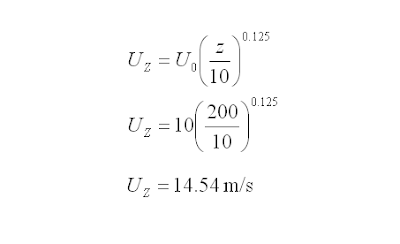
UZ = 14.54 m/s
Wind speed at flare tip with return duration stay as 60 minutes = 14.54 m/s
Related Topic
Subscribe FREE - Chemical Processing
As discussed in earlier post "Estimate Wind Speed At Flare Tip At Different Height", correct wind speed at flare tip (elevated flare) is important in order to obtain correct estimate of radiation level and unburnt component concentration at downwind location, determination of minimum vapor flow to avoid flame-out and performance of pilots. A rather complicated equations may be used to estimate wind speed at different height.This will present a rather simple relation to estimate the wind speed. The following equation may be considered.

UZ = Wind speed at Z m at return duration of t0 hour (m/s)
U0 = Wind speed at specified height of 10m at return duration of t0 hour (m/s)
t0 = Wind speed at return duration i.e. 60 minutes, 1 minutes, etc
Z = Flare stack height (m)
K = Field data derived parameter (may use 0.125)
Example :
A flare stack with height of 200m, expose to wind speed (at 60 minutes return duration) of 10 m/s measured at 10m from grade. Determine wind speed at flare tip if the return duration stay as 60 minutes.
Solution (a)
Z = 200 m
U0 = 10 m/s

UZ = 14.54 m/s
Wind speed at flare tip with return duration stay as 60 minutes = 14.54 m/s
Related Topic
- Estimate Wind Speed At Flare Tip At Different Height
- Assess AIV with "D/t-method" with Polynomial PWL Limit Line
- Model Fix Pressure Device in FLARENET
- Several Criteria and Constraints for Flare Network - Process
- Several Criteria and Constraints for Flare Network - Piping
- Provide More than One Flare KOD in SERIES
Labels: Environment, Flare
Saturday, June 13, 2009

Subscribe FREE - Chemical Processing
Chemical Engineering has shared a new FAYF. This FAYF is related Choosing Control System.Process engineer - Why you need to know Control System
Choosing a control system is not a process engineer task. It is typically Instrumentation and Control engineer task. However, understand what is control system, how many type of control system, how a control system works, differences between control system, etc may be important to a process engineer as process engineer define main control objective in Piping & Instrumentation Diagram (P&ID) to achieve the control target and preparation of System Control Narrative so that Control engineer can further develop the control logic.
Typical Control System
Two main type : Distributed Control System (DCS) and Programmable Logic Control System (PLC). A DCS is designed for process control with refinery control origins whilst a PLC is designed for machine or motion control with car factory relay panel origins. While PLCs are sometimes used for process-control applications, there are some trade-offs in terms of degree of programming, robustness and operational suitability.
Control System Characteristic
Distributed control system (DCS)
1. Gregg, J., Control System Selection, Chem. Eng., August 2002, pp. 62–66.
2. Bohan, J., Industry Solutions Manager, Honeywell Process Solutions (Phoenix, Ariz.), personal communication, Apr. 6, 2009.
Download
Note :
*This FAYF is only available FREE to Chemical Engineering Magazine registered user. Login required. Subscribe FREE CE, click here.
** Download immediately as article available FREE within short period only. Do not wait.
*** Found lost link or unable to download, may contact me...
Related Topic
Choosing a control system is not a process engineer task. It is typically Instrumentation and Control engineer task. However, understand what is control system, how many type of control system, how a control system works, differences between control system, etc may be important to a process engineer as process engineer define main control objective in Piping & Instrumentation Diagram (P&ID) to achieve the control target and preparation of System Control Narrative so that Control engineer can further develop the control logic.
Typical Control System
Two main type : Distributed Control System (DCS) and Programmable Logic Control System (PLC). A DCS is designed for process control with refinery control origins whilst a PLC is designed for machine or motion control with car factory relay panel origins. While PLCs are sometimes used for process-control applications, there are some trade-offs in terms of degree of programming, robustness and operational suitability.
Control System Characteristic
Distributed control system (DCS)
- Continuous control
- Parameters change frequently
- Sequence capability in batch process
- Operators intervention
- Integration with other applications
- Robust control
- Multiple controllers interaction
- High availability
- Historical data collection
- High speed processing
- Discrete application (digital inputs/outputs)
- Application predominantly in machine/motion control
- Application do not change frequently
- SCADA architectures with PLCs
- Capability of operators intervention & decision
- Ladder logic is effective way to handle logic
- Separated application with small amount of I/O
1. Gregg, J., Control System Selection, Chem. Eng., August 2002, pp. 62–66.
2. Bohan, J., Industry Solutions Manager, Honeywell Process Solutions (Phoenix, Ariz.), personal communication, Apr. 6, 2009.
Download
Note :
*This FAYF is only available FREE to Chemical Engineering Magazine registered user. Login required. Subscribe FREE CE, click here.
** Download immediately as article available FREE within short period only. Do not wait.
*** Found lost link or unable to download, may contact me...
Related Topic
Labels: Control
Friday, June 12, 2009
Display problem ? Click HERE

FREE Chemical Engineering Digital Issue for June 2009 has been released !
Chemical Engineering has just released FREE June 2009 issue. If you are subscriber of Chemical Engineering, you should have received similar notification.
***********************
Interesting articles for this month :
Dry Tray Pressure Drop Of Sieve Trays
This new correlation matches most commercial trays
Renewable Feedstocks : Trading Barrels for Bushels
Efforts to boost conversion rates and yields and improve separation efficiency are helping, but obstacles remain
Strengthening The Weakest Link
New materials and designs help seals and gaskets evolve into components that can overcome today’s CPI challenges
FAYF : Specialty Metals
This one-page guide details the factors to consider when evaluating specialty metals as a material of construction
Beyond Flowmeter Selection : Consider Some of the Most Overlooked Criteria
The whole product-lifecycle approach encompasses more
Avoiding Static Sparks In Hazardous Atmospheres
Relatively simple steps can be taken to mitigate risks associated with static electricity in process plants
Vibratory Feeders And Conveyors: Useful Selection Tips
Ongoing advances in technology have helped these systems overcome key shortcomings of earlier designs
***********************
TIPS
If you are subscriber, you may access previous digital releases. Learn more in "How to Access Previous Chemical Engineering Digital Issue".
If you yet to be subscriber of Chemical Engineering, requested your FREE subscription via this link (click HERE). Prior to fill-up the form, read "Tips on Succession in FREE Subscription".
Related Post
- How to Access Previous Chemical Engineering Digital Issue
- Tips on Succession in FREE Subscription
- 3 Most Important & FREE Magazines That I Read...
- Non - Technical Quick References for a Chemical & Process Engineers
- More You Share More You Learn
- Knowledge is Own by Everyone but Not Someone
Labels: E-Doc, Education, Learning
Thursday, June 11, 2009
Display problem ? Click HERE
Recommended :
Flare is commonly installed in oil and gas process plant to burn hydrocarbon and/or toxic gas to avoid formation of combustible mixture, to minimize green house effect (GHE), to minimize health hazards to personnel on site, etc. There are several earlier posts related to Flare :
- Quick Estimate Flare Stack Diameter
- Estimate Subsonic Flare Tip Pressure Drop With Graph Derived Correlation
- Quick Estimate Flare Tip Pressure Drop
- Flare Tip Type Quick Selection Chart
- ANSI/API Std 537 / ISO 25457 2nd edition, Dec 2008 is Released
- Guideline on Quick Determination of Flare Stack Support Type
- Flare Smokeless Ringlemann Chart
- Must Read Flare Handbook
- FLARE combustion efficiency
- Quick Estimate Ground Level Unburnt Flammable Gas For Vent Pipe or Flame-out Flare Stack
- Elevated Flare (SI Unit) Datasheet
- Enclosed Flare (SI Unit) Datasheet
Wind speed affects flare performance at least in few ways :
- Wind drag flame to downwind, lower the flame center and radiation level of downwind receptor
- Wind carry unburnt component to downwind
- Wind potential put-off flame on flare under low gas flow and pilot
Wind speed change with flare height
One of characteristic of wind speed is wind speed increase with height from grade. Thus, higher the flare stack, flare tip will expose to higher wind speed. Generally wind map will be obtained from local authority or organization. The wind map may be measured at specific height i.e. 10m from grade.
In case flare stack height is different than wind speed at specific height, how shall an engineer determine wind speed flare tip ?
Corrected wind speed (without return duration correction)

Where
UZ = Wind speed at Z m at return duration of t0 hour (ft/s)
U0 = Wind speed at specified height of 10m at return duration of t0 hour (ft/s)
t0 = Wind speed at return duration i.e. 60 minutes, 1 minutes, etc
Z = Flare stack height (ft)
Corrected wind speed (with return duration correction)

Where
t = Wind speed at return duration i.e. 60 minutes, 1 minutes, etc (different than t0 )
Example :
A flare stack with height of 200m, expose to wind speed (at 60 minutes return duration) of 10 m/s measured at 10m from grade. Determine wind speed at flare tip if (a) the return duration stay as 60 minutes (b) return duration change to 1 minute.
Solution (a)
Z = 200 m = 200 x 32.8 ft
UZ = 10 m/s = 10 x 32.8 ft/s

UZ = 41.7 ft/s = 12.7 m/s
Wind speed at flare tip with return duration stay as 60 minutes = 12.7 m/s
Solution (b)

uZ,t = 44.8 ft/s = 13.66 m/s
Wind speed at flare tip with return duration at 1 minutes = 13.66 m/s
Related Topic
- Assess AIV with "D/t-method" with Polynomial PWL Limit Line
- Model Fix Pressure Device in FLARENET
- Several Criteria and Constraints for Flare Network - Process
- Several Criteria and Constraints for Flare Network - Piping
- Provide More than One Flare KOD in SERIES
Labels: Environment, Flare
Wednesday, June 10, 2009
Display problem ? Click HERE
Recommended :
- Subscribe FREE - Processing Magazine
- Tips on Succession in FREE Subscription
 A webinar"Convert Complexity into Clarity: Performance Management and Optimization in Process Manufacturing" targeted to assist you and your company simplify disparate systems, inconsistent processes and suspect data, increased operation performance including less waste, more through-put, less downtime and fewer people. It is FREE and open for registration now. As companies look to drive out waste from manufacturing operations, understanding current performance is essential. In many cases, this first step of clarity is the most challenging part of the continuous improvement process.
Disparate systems, inconsistent processes and suspect data all add to the complexity of “gaining that first foothold” of operations performance management. How these challenges are addressed directly affects both the immediate benefits and ongoing continuous improvement.
During this free webcast on June 24th 2009 at 11 am Eastern Daylight Time, speaker will :
Brought to you by : Processing magazine
Sponsored by : SAP
Related Post
- Subscribe FREE - Processing Magazine
- Tips on Succession in FREE Subscription
A webinar"Convert Complexity into Clarity: Performance Management and Optimization in Process Manufacturing" targeted to assist you and your company simplify disparate systems, inconsistent processes and suspect data, increased operation performance including less waste, more through-put, less downtime and fewer people. It is FREE and open for registration now. As companies look to drive out waste from manufacturing operations, understanding current performance is essential. In many cases, this first step of clarity is the most challenging part of the continuous improvement process.Disparate systems, inconsistent processes and suspect data all add to the complexity of “gaining that first foothold” of operations performance management. How these challenges are addressed directly affects both the immediate benefits and ongoing continuous improvement.
During this free webcast on June 24th 2009 at 11 am Eastern Daylight Time, speaker will :
- Cover strategies for accelerating performance management
- Explain how current systems and processes can contribute or detract from your performance management strategy
- Discuss examples from leading companies who experienced rapid innovation and year-over-year value using a proper foundation of performance management with an agile platform
- ‘Question and Answer’ period with your peers in plants across the country.
Brought to you by : Processing magazine
Sponsored by : SAP
Related Post
- Engineering Advancement is Critical...
- Chemical Engineer Average Salary From 2005 - 2009
- 3 Most Important & FREE Magazines That I Read...
- Don't miss CHEMICAL ENGINEERING Supplementary Issue in Chinese...
- Non - Technical Quick References for a Chemical & Process Engineers
Labels: Education, Learning, NEWS
Monday, June 8, 2009
Display problem ? Click HERE
Recommended :
- Subscribe FREE - Processing Magazine
- Tips on Succession in FREE Subscription
High frequency acoustic excitation downstream of pressure reducing device and potential of downstream piping failure on Acoustic Induced Vibration (AIV) has raised concern in many plant design. Earlier post "Extra Attention to Common Point and Similarity on AIV Failure" has discussed the common points and similarity of AIV such as typical failure location, system experienced failure in the past, failure time & period and Mach no. An engineer assessing AIV shall pay extra attention in these factors.
- Subscribe FREE - Processing Magazine
- Tips on Succession in FREE Subscription
High frequency acoustic excitation downstream of pressure reducing device and potential of downstream piping failure on Acoustic Induced Vibration (AIV) has raised concern in many plant design. Earlier post "Extra Attention to Common Point and Similarity on AIV Failure" has discussed the common points and similarity of AIV such as typical failure location, system experienced failure in the past, failure time & period and Mach no. An engineer assessing AIV shall pay extra attention in these factors.Earlier post "Assess AIV with "D/t-method "has presented a Sound Power level (PWL) limit line (logarithm line) to assess the possibility of Acoustically Induced Fatigue failure based on D/t method. Nevertheless, there is still some concern on the area where there is no published data shows the possibility of AIV failure (shown as pink triangle area in below image). Eisinger PWL limit line and Logarithm PWL limit line consider this area is non-failure.

Taking conservative approach, this area may be defined as area potentially failure until more real field or experiment data available. Therefore, a new Polynomial PWL limit line is proposed.
PWLlimit =C4.r4 + C3.r3 + C2.r2 + C1.r + C0
Where
PWLlimit = Maximum allowable PWL at Pipe diameter D meter, (dB)
r = 1000D/t
D = Pipe Outside diameter (m)
T = Pipe wall thickness (mm)
C4 = 0.000000032
C3 = 0.000023
C2 = 0.0057
C1 = 0.691
C0 = 192
Refer following graph. New polynomial presented as violet line.
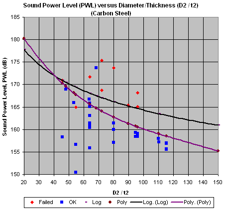
Note :
1) A "failure" point (0.3m, 165dB) is below curve. It is failed on bad welding. No further failure after good welding.
2) Red point are "failure" point and Blue point are "No failure" point
3) May be used for 0.2m < D < 0.9m. Use at risk for D < 0.2m and D > 0.9m
This line may be used to assess potential failure of piping downstream of pressure reducing device. Any point above this line potentially fail on AIV, piping treatment or redesign required to minimise the risk of AIV failure. This will be discussed in future...
Related Topic
- Assess AIV with "D/t-method"
- Extra Attention to Common Point and Similarity on AIV Failure
- Piping Excitation When Expose to Acoustic Energy
- Acoustic Induced Vibration (AIV) Fatigue
- Sound Power Level (PWL) Prediction from AIV Aspect
- Several Criteria and Constraints for Flare Network - Piping
- Quick Estimation of Noise Level Across Pressure Reducing Device
- Noise Level Across Pressure Reducing Device For Different Pipe Wall Thickness
Sunday, June 7, 2009
Display problem ? Click HERE
Modeling & Simulation is commonly used is Chemical and Process engineering as a tool to analyze, understand and predict behavior and performance of a system. What is meaningful way of putting System, Model, and Simulation in an appropriate perspective ? System, Model and Simulation may be viewed as :
- System - A system exists and operates in time and space.
- Model - A model is a simplified representation of a system at some particular point in time or space intended to promote understanding of the real system.
- Simulation - A simulation is the manipulation of a model in such a way that it operates on time or space to compress it, thus enabling one to perceive the interactions that would not otherwise be apparent because of their separation in time or space.

Modeling & Simulation: The Return on Investment (ROI) in Materials Science
The use of Modeling & Simulation software suggests a cumulative ROI of $3 to $9 for every $1 invested in scientific research. The mechanisms for these gains are:
- Increased experimental efficiency leading to the reduction of direct research costs
- Efficiency gains leading to broader and deeper exploration of solutions and new products
- Financial gains by improving time to market for new products or line extensions
- Revenue gains from the rescue of stalled product development projects
- Risk management through safety testing and failure analysis
Related Post
- Engineering Advancement is Critical...
- Chemical Engineer Average Salary From 2005 - 2009
- 3 Most Important & FREE Magazines That I Read...
- Non - Technical Quick References for a Chemical & Process Engineers
- R&D engineer, Academician and Student...Don't miss this !
- More You Share More You Learn
- Knowledge is Own by Everyone but Not Someone
Friday, June 5, 2009
Display problem ? Click HERE
Chemical & Process Technology In Twitter Now...!
 Earlier post "Quick Estimation of Noise Level Across Pressure Reducing Device", discussion has been focused on estimation of Noise level across pressure reducing device i.e. control valve, pressure relief valve, restriction orifice, etc based on generated internal acoustic energy and transmission losses. The table presented in this post is typical wall thickness for Schedule STD. Increases in wall thickness (e) will results higher transmission loss and lower noise level is expected. Besides, magnitude of transmission loss is also depends to line diameter (D). How to relates transmission loss with wall thickness for different diameter ?
Noise Level Estimation
Noise level at 1 meter from a pressure reducing device can be estimated from Sound Power Level (PWL) as discussed in "Sound Power Level (PWL) Prediction from AIV Aspect". The Sound Power Level will be transmitted across the pipe wall and emitted to atmosphere. There will be noise correction when Sound power is transmitted across pipe wall (metal).
Noise level at 1 meter from a pressure reducing device,
L1m = PWL - LA
where
PWL = Sound Power Level (from Sound Power Level (PWL) Prediction)
LA = Noise correction (dB)
Noise Correction
The noise correction is subject to wall thickness and pipe size. Thicker wall will result higher noise correction. Following are sets of noise correction equation for different pipe size and wall thickness.
For Nominal Diameter equal to 750 (30 inches) and smaller,
LA = C3.e3 + C2.e2 + C1.e + C0 ......[1]
For Nominal Diameter 900 (36 inches) and above,
LA = C1.Ln (e) + C0 .....[2]
Where
e = Pipe wall thickness (mm)
C0, C1, C2, C3 = Parameters
e = Pipe wall thickness (mm)
C0, C1, C2, C3 = Parameters
| Parameter for Noise Correction | |||||
| Nom.Dia. (Inch) | Eq. | C3 | C2 | C1 | C0 |
| 25 | 1 | 0.0580 | -1.2556 | 11.6751 | 26.0942 |
| 50 | 1 | 0.0319 | -0.8039 | 8.8155 | 25.7428 |
| 100 | 1 | 0.0070 | -0.3107 | 5.6726 | 25.7582 |
| 150 | 1 | 0.0046 | -0.2351 | 4.8724 | 24.2083 |
| 200 | 1 | -0.0002 | -0.0376 | 2.3897 | 31.0074 |
| 250 | 1 | 0.0023 | -0.1395 | 3.1106 | 28.5213 |
| 300 | 1 | 0.0013 | -0.0949 | 2.5482 | 29.9195 |
| 350 | 1 | 0.0012 | -0.0858 | 2.4017 | 29.2649 |
| 450 | 1 | 0.0008 | -0.0660 | 2.1185 | 30.5846 |
| 600 | 1 | 0.0003 | -0.0371 | 1.5550 | 32.7016 |
| 750 | 1 | 0.0007 | -0.0523 | 1.7118 | 31.1754 |
| 900 | 2 | - | - | 6.9521 | 27.3305 |
| 1050 | 2 | - | - | 10.4282 | 18.4957 |
Example
A pressure control valve (PV) passing 100,000 kg/h of gas with molecular weight (MW) of 22. The inlet condition is 87 barg and 50 degC and downstream pressure is about 7 barg. The pipe diameter is 18 inch with wall thickness of 9.53mm, estimate noise level at 1 m from PV.
PWL = 10 x Log [((87-7) / (87+1.01325))^3.6
x (100,000 / 3600)^2
x ((50+273.15)/22)^1.2]
+ 126.1
PWL = 167.5 dB
For 18 inches, equation [1] will be used.
LA = C3.e3 + C2.e2 + C1.e + C0
LA = 0.0008 x9.533 -0.0660x9.532 + 2.1185 x 9.53 + 30.5846
LA = 45.5 dB
Noise level at 1m,
L1m = PWL - LA
L1m = 167.5 - 45.5
L1m = 122 dBA
Related Topic
- Quick Estimation of Noise Level Across Pressure Reducing Device
- Assess AIV with "D/t-method"
- Extra Attention to Common Point and Similarity on AIV Failure
- Piping Excitation When Expose to Acoustic Energy
- Acoustic Induced Vibration (AIV) Fatigue
- Sound Power Level (PWL) Prediction from AIV Aspect
- Several Criteria and Constraints for Flare Network - Piping
- Flow Element (FE) Upstream or Downstream of Control Valve (CV) ?
Labels: Air Pollution Control, AIV, Safety
Monday, June 1, 2009
Display problem ? Click HERE
Chemical & Process Technology In Twitter Now...!
A recent survey (Jan 2009) conducted by HART Research Institute indicates that (Americans' opinion) most important aspects in engineering including green energy, improving infrastructure, and clean water. Engineering advancement is critical in society development and have high expectation on engineering. However, they have little understanding about what engineer is doing. This has lead to many young people lose their interest on Engineering. They have the opinion that other countries such as Japan or China may is better able to deliver engineering advance. To maintain present technology leader in the world, education is one of the element. Read more in presentation.What do you think ?
Related Post
- Chemical Engineer Average Salary From 2005 - 2009
- 3 Most Important & FREE Magazines That I Read...
- Don't miss CHEMICAL ENGINEERING Supplementary Issue in Chinese...
- Non - Technical Quick References for a Chemical & Process Engineers
- R&D engineer, Academician and Student...Don't miss this !
- More You Share More You Learn
- Knowledge is Own by Everyone but Not Someone
